Introduction
Composite Indicators (CI) are a quantitative measure that aggregate multi-dimensional data into a single index. Differently from other aggregation methods as Principal Components Analysis (PCA) or Factorial Analysis (FA) they are not entirely data driven and they are compiled in order to communicate a concept. Mostly used in social or policy evaluation, they allows for a single and direct comparison between their units. Gamers commonly and intuitively use this tool when talking about tier list. In a card game like Hearthstone (HS) a simple but known example of CI is the Meta Score from viciousSyndicate (vS).
In Legends of Runeterra (LoR) we created a similar CI defined as LoR-Meta-Index (LMI)1. The index didn’t just try to replicate the vS Meta Score but tried to adjust it to the LoR data and its differences from HS. A limitation of the proposed index is it’s composed by only two variables: play-rates and win-rates. While they are the most important variables of performance of a deck, they don’t fully catch the complexities on the meta-game performances. This can be solved by adding other variables to the index and a natural candidate is the ban-rate of a deck (in a contest of BoX matches).
An experiment to add the ban-rate was done earlier this year, for ‘Rise of the Underworld - Seasonal Tournament’ report2.
The inclusion of such variable, was done without checking all the proper steps so that we wouldn’t compromise the quality of the CI. In this article we introduce in more detail the concept and framework of a CI and how to add the the information of the ban rates and their results.
Following the necessary steps, the proposed variation of the LMI partially contradicts the expected theoretical-framework requiring an higher level of complexity to reach the aimed .
Data
Data are taken from the Seasonal tournaments ‘Guardian of the Ancient’ and ‘Rise of the Underworld’ Open Rounds.
The Open Rounds are the are organized in a series of nine Bo3 Matches with open lists and a ban phase before the start of the games. The smaller amount of games from the Asian shard/server is allegedly because of the fewer players taking part of it3
Not all information about the tournament can be derived from the API. There is no direct data about the chosen ban deck or the entire line-up brought by a player at this have to be extracted by aggregating the metadata of games from a single match and all matches played during that day.
We only consider the decks that appears in the cases of a full-line-up and whose we can extrapolate the banned deck.
To evaluate win-rates on the ladder, as additional source, we includes Ranked games from Master players (at least one of the two players being Master) from up to two weeks before the start of the first game of the Seasonal (because of the time zone, two weeks, before the start of the Asian Seasonal).
| Bo3 Data | ||
|---|---|---|
| Matches by Server | ||
| Characteristic | Seasonal - Guardian of the Ancient, N = 20,6371 | Seasonal - Rise of the Underworld, N = 20,5111 |
| server | ||
| americas | 9,126 (44%) | 9,018 (44%) |
| asia | 2,457 (12%) | 2,421 (12%) |
| europe | 9,054 (44%) | 9,072 (44%) |
| Bo3 Data from Seasonal Open Rounds - Rise of the Underworld Open Rounds Matches - games extracted with Riot API | ||
|
1
n (%)
|
||
Example and part of the raw-data used can be found in Appendix ??)
Methods
Composite Indicators - A Better Introduction
The LMI is a composite indicator (CI) and in a previous article we introduced the tool we gave a brief explanation about how to create them. Here, we want to give a better and more complete overview of the tool.
For a manual on CI, a commonly referred guide is from the Joint Research Centre (JRC) of the European Commission: Handbook on Constructing Composite Indicators - METHODOLOGY AND USER GUIDE. In that guide building a composite indicator requires the following 10 steps:
- Theoretical Framework
Provide the basis for the selection and combination of variables into a meaningful composite indicator under a fitness-for-porpuse principle (involment of experts and stakeholders is envisaged at this step)
What is the concept that the CI wants to convey? Of what characteristics is it made and what variable can express them? This steps is all about setting the definition of what needs to be created.
- Data selection
Should be based on the analytical soundness, measurability, coverage and relevance of the indicators to the phenomenon being measured and relationship to each other. The use of proxy variables should be considered when data are scarce (involvement of experts and stakeholders is envisaged at this step)
When defining the CI structure there is also the need to maintain a coherent structure. This means, among other, that values in the same sub-dimension should all follows the same direction. In an increase of a variable imply an increase in the final value of the sub-dimension index then all the other variables should be same.
Example: if we have a sub-dimension index related to “quality of life” containing life expectancy and child mortality, the higher the value of life expectancy the better and higher the final index should be. But, for the values of child mortality it is the opposite, the smaller the value, the better it is. In this case it’s not a problem as a common practise is to just use the opposite values by changing the sign as it is a linear transformation and the smaller the value of child mortality (with opposite sign) the better it is in evalutating “quality of life”.
The ‘polarity’ of an individual indicator is the sign of the relation between the indicator and the concept to be measured. For example, in the case of well-being, “Life expectancy” has positive polarity, whereas “Unemployment rate” has negative polarity. I
- Imputation of missing data
Is needed in order to provide a complete dataset (e.g by means or multiple imputation).
In the real world rarely the available data are complete (and this article is no exception). If the missing value are MCAR (Missing Completely At Random) then there would be no problem to just remove the rows with missing values but this is not always the case and sometimes we can’t just remove units as they too important and so we must try to impute the missing values without compromising the end results or estimate these values to be as near as possible as what we would have obtain as the “true” value (not compromising the quality and trying to estimate the best imputation are not the same problem).
Dealing with outliers is also part of this step. In our case it’s related to the minimum amount of games to require to a deck.
- Multivariate analysis
Should be used to study the overall structure of the dataset, assess its suitability, and guide subsequent methodological choices (e.g. weighting aggregation).
Sometimes the framework is not enough to guide our decision and variables may actually behave differently from our exceptions. This step is about checking the underlying structure of the data, helps identify groups and evaluate statistically evaluated structure of the data set to the theoretical framework and discuss potential differences.
In this article this will be done when looking at the correlations among our variables.
- Normalization
Should be carried out to render the variables comparable
As this steps was invested with care in the previous article, we will maintain the choice for using a quantile normalization for our data.
While it’s possible to use different normalization for the same CI at different groups of variables, it’s not a recommended practise.
- Weighting and aggregation
Should be done along the lines of the underying theoretical framework
This steps mostly intertwined with the the Multivariate analysis as it can highlight
Like the normalization step, this step too was was invested with care in the previous article and we will maintain the choice for using an harmonic mean when aggregating our data. It is possible to use different aggregation method for the same CI if it’s justified (like for compensability)
- Uncertainty and sensitivity analysis
Should be undertaken to assess the robustness of the composite indicator in terms of e.g. the mechanism for indulging or excluding an indicator, the normalization scheme, the imputation of missing data, the choice, the choice of weights, the aggregation method
This is an highly complex step that will be left for future articles.
- Back to the data
Is needed to reveal the main drivers for an overall good or bad performance. Trasparency is promordial to good analysis
As it can be done better with the results of a uncertainty and sensitivity analysis, this steps too will be left for the future.
- Links to other indicators
Should be made to correlate the composite indicator (or its dimension) with existing (simple or composite) indicators as well as to identify linkages through regressions.
This can be done when comparing the result of Balco’s Meta-Score which applies the same algorithm by vS but is not part of this article as we would also include the opinion of third-party experts (some high level players) to evaluate the different CI performances.
- Visualization of the results
Should receive proper attention, given that the visualization can influence (or help to enhance interpretability)
While not the only choice we will maintain for now the same plot strcture used up until now in the meta-reports and the previous LMI article.
When creating for the first time a CI these 10 steps aren’t done in a strict sequential order, so in this article we will sometimes return to what is are previous steps compared to the one we are mainly referring in a section of the article.
The LMI Composite Indicator
Base LMI
The basic LMI is made by aggregating play-rates and win-rates and its creation was was inspired by seeing the meta score on vS.
While the base raw data are from the same concept, they are combined in a different way.
From their F.A.Q.
Q: What is the meaning of the Meta Score and how do you compute it?
The Meta Score is a supplementary metric that measures each archetype’s relative standing in the meta, based on both win rate and prevalence, and in comparison to the theoretical “best deck”.
How is it computed?
…
We take the highest win rate recorded by a current archetype in a specific rank group, and set it to a fixed value of 100. We then determine the fixed value of 0 by deducting the highest win rate from 100%. For example, if the highest win rate recorded is 53%, a win rate of 47% will be set as the fixed value of 0. This is a deck’s Power Score. The range of 47% – 53%, whose power score ranges from 0 to 100, will contain “viable” decks. The length of this range will vary depending on the current state of the meta. Needless to say, it is possible for a deck to have a negative power score, but it can never have a power score that exceeds 100.
We take the highest frequency recorded by a current archetype in a specific rank group, and set it to a fixed value of 100. The fixed value of 0 will then always be 0% popularity. This is a deck’s Frequency Score. A deck’s frequency score cannot be a negative number.
We calculate the simple average of a deck’s Power Score and Frequency Score to find its vS Meta Score. The vS Meta Score is a deck’s relative distance to the hypothetical strongest deck in the game. Think of Power Score and Frequency Score as the coordinates (x, y) of a deck within a Scatter Plot. The Meta Score represents its relative placement in the plane between the fixed values of (0, 0) and (100,100).
If a deck records both the highest popularity and the highest win rate, its Meta Score will be 100. It will be, undoubtedly, the best deck in the game.
While for the LMI:
Only decks with at least 200 games are considered. A similar filter is most likely being applied by vS too, we just don’t know the values for the cut-off
Play-rates and win-rates are normalized with a quantile normalization into a Freq-Index and a Win-Index
Freq-Index and a Win-Index are aggregated by an harmonic mean of equal weights into the LMI
The reasoning behind these choices compared to other options can be found in the LMI - early concept article.
Adding Banrate Information
As the number of variables increase from the two of the base-LMI to three we now have more options as to combine them. Normally, this doesn’t mean that each possible choice should be evaluated, the definition we want to communicate should guide our choices and so the characteristics of our variables, e.g. we don’t add a variable of Life expectancy in a sub-dimension of ‘Infrastructure quality’
When creating the LMI we described it as a measure of performance of a deck and as definition of performance of a deck as:
The performance of a deck is defined by its own strength and popularity inside the metagame.
The definition of performance is probably not be as functional as it should as it seems a bit limiting in what it means. Yet, the term performance still remains appropriate.
What information can be added to the index? An easy inspiration can be taken from Riot’s main games: League of Legends (LoL)
In LoL a common value to describe the performance of a champion, in in addition to play-rates and win-rates is the ban-rate of a champion.
The most infamous value of the ban-rate was 95% ban-rate of Kassadin in S3. If we consider the definition of performance given earlier we can see that the ban-rate doesn’t fir perfectly strength or popularity in the metagame but it is more a case in the middle. It can seen as an aspect of strength as people don’t want to deal with it, so banning it, but it can be as an aspect of popularity or better yet a more general presence as while it may have not been played it sort of lingers in the match. The banned champion was not present directly in the match but with its spirit (the ban).
In the context of LoR such information can be added once we consider BoX data, currently only Bo3 with the easiest example being the Seasonal Tournaments and a possible way to define it is:
- Ban Rate - ratio between the number of bans and the number of matches of a deck.
\[\begin{equation} BanRate = \frac{\#ban}{\#match} \end{equation}\]
Example: 2 Line-Ups contained a Teemo/Ezreal deck, both played all 9 matches and Teemo/Ezreal was banned respectively 3 and 6 times; the ban rate would be \(\frac{(3+6)}{(9+9)} = 50\%\)
As the variable is deemed appropriate for the LMI purpose the following step is to define the structure of the LMI to account for the new variable.
With just three variables the possible ways to combine them are exactly three as shown in Fig:1, Fig:2 and Fig:3
Figure 1: (1/3) Possible theoretical framework for the LMI - All the variables are part of their own subdimension
Figure 2: (2/3) Possible theoretical framework for the LMI - retaining two main subdimension of the base LMI, ban-rate and win-rate are both used to measure the ‘strenght’ of a deck
Figure 3: (3/3) Possible theoretical framework for the LMI - retaining two main subdimension of the base LMI, ban-rate and playrate are both used to measure the ‘presence’ of a deck
Each different structure correspond to a different way to see the ban-rate relationship with the other variables.
In the first structure it is considered a different characteristic altogether in comparison to play-rates and win-rates.
In the second structure the ban-rate of a deck is considered a part of its ‘strength’, the higher it is the more it means that players don’t want to deal with it be it for play-patterns, expected win-rates, or other reasons one may have.
In the third structure the ban-rate of a deck is considered a part of its ‘presence’, it may have not been played, but like in the Kassadin example before, it’s lingering in the matches as an unseen factor that is still influential to the results. After all the ban or not of a deck, so if it takes an active or passive role in a match can heavily influence the remaining Match Ups.
While the second structure may seems the more intuitive choice, none of these strctures are the one proposed at the end. This is because of the results we found during the statistical analysis.
Statistical Analysis
In this section we describes how the analysis was done in its entirely and not just the final version of the steps to do in order to create the LMI. This is so to highlight some of the results we found and how we add the account for them.
Correlation
To assess which structure should be used we need to check the relationship between variables. This can be done by looking at their correlations.
Using all the data and calculating the correlation would be wrong, as, as showed in the previous LMI article it is better to limit the analysis to a smaller pool of decks with a sufficient amount of games.
At the Seasonal Tournament the number of games in total is overall small compared to the number of decks played so we tried a series of possible cut-off as min number of games played and find a compromise between not eliminating too many decks and having enough data to have quality results.
We tried to decide the min number of games required by looking at the amount of remaining decks we would have. The effect of different choices can be seen in Tab:1.
Note: it’s the number of decks with also no missing values, as in the 296 decks there is 1 with no mean ban-rate even at cut-off of zero, the overall number is reduced by one.
Table 1: Cut-off Table
| minGames | #Deck |
|---|---|
| 0 | 295 |
| 10 | 145 |
| 30 | 79 |
| 50 | 52 |
| 100 | 37 |
| 200 | 29 |
| Amount of remaining Decks depending on the required min amount of Games |
|
At the first glance, the 200 games used during the meta-reports seems excessive as it reduce the decks to 1/10th, 10 games is probably not enough as the win-rates would be too unstable making us gravitating mostly on 30,50,100 but we will truly decide being guided by the correlation results as shown in Tab:2.
Table 2: Correlation Table at different cut-off
| Correlation | 0 | 10 | 30 | 50 | 100 | 200 |
|---|---|---|---|---|---|---|
| WR/playrate | 0.07 | 0.12 | 0.18 | 0.16 | 0.13 | 0.08 |
| meanBan/playrate | 0.09 | 0.24 | 0.29 | 0.33 | 0.28 | 0.24 |
| meanBan/WR | -0.02 | 0.09 | -0.07 | -0.03 | -0.08 | -0.02 |
| Correlation between the three raw variables on different amount of required min amount of Games | ||||||
The resulting correlations took us by surprise in a first moment. Not only the variable with the higher correlation to the ban-rate is the play-rate and not the win-rate (the expected initial result) but the correlation with win-rate seems to be negative. This is not strange, in Bo3 setting after the bans each player tries to enforce the best match-ups among the remaining decks so it easier to have bad match-ups even for highly-performing decks on the ladder. This made us question whatever to aggregate the ban-rate with play-rate, so the structure in Fig:3. What we actually did was to consider:
- If the ban-rate of a deck during the Seasonal is negative correlated its win-rate it’s probably because many brought counter line-ups to popular and strong decks. So it would also means that the ban-rate is also correlated to the performance of a decks in the ladder before the tournament.
We tried to see if this is the case by looking at the correlation of the ban-rates with not just the win-rates at the Seasonal but also the win-rates from the ladder up to two weeks before the tournament starts. Since the aggregation is not done with the raw values but the normalized transformation the correlation is calculated after the normalization step using the quantile normalization as done in the previous iteration of the LMI. In addition, not to be affected by the particular tournament chosen this is why we also used the data from the ‘Seasonal Tournament - Guardian of the Ancient’ when the case-study was aimed to compute the LMI for the ‘Rise of the Underworld’ edition. As seens in Fig:4 this was a crucial choice as the relationship of the ban-rates with the Seasonal win-rates can change radically. In the June tournament the metagame was more polarized and this probably affected the correlations.
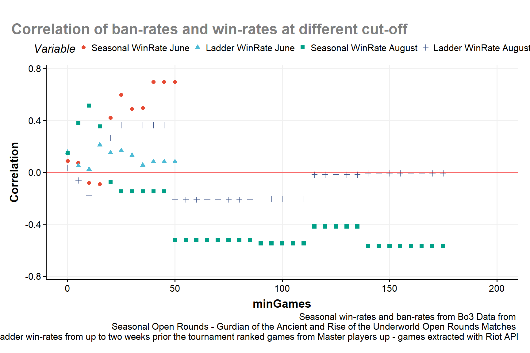
Figure 4: correlation of Seasonal Win-Rates and Ladder Win-Rates with the Ban-Rates at different benchmarks of minimum amount of games for each deck
How to continue was the hardest part of the analysis. The correlation of ladder win-rates have a strong positive orientation with the ban-rates while the correlation with the Sesonal win-rates is more unstable and tends to be negative for certain value. If we wanted to use the structure of Fig:1 or Fig:2 than our problem would have to aggregate variables with different orientations. While this is not a rule one must always follows in the cases mentioned this would negatively impact the quality of the LMI. We would have for sure that an high value of a deck would decrease the win-rate index and to have an high LMI we may not want an high ban-rates as it’s increase may decreae the win-rate. It would be harder to have decks with high LMI and high values of both win-rates and ban-rates. At the same time, can we really say the strength of the deck is the one we measured if the win-rates we observe seems to be a consequence of the metagame from the ladder and the high performances in Bo1 that is reflected by high ban-rates as to suggest people don’t want to deal with decks they in the ladder they found are difficult to deal with unless the line-up can handle them?
The solution proposed is to use a win-index that is not created from just the Seasonal win-rates but also the ladder win-rates to include both informations and having the ladder value reduce if not remove the negative correlation of the Seasonal value. Both for this to work we have to check a couple of conditions:
Win-rates from Seasonal and ladder needs to be correlated and the orientation shouldn’t change depending on the tournament, which is a legit worry after seeing the previous figure. A positive correlation can be found and seen in Fig:5.
The aggregated win-rates have works better as a component to aggregate with ban-rates. The results can be seen in Fig:6.
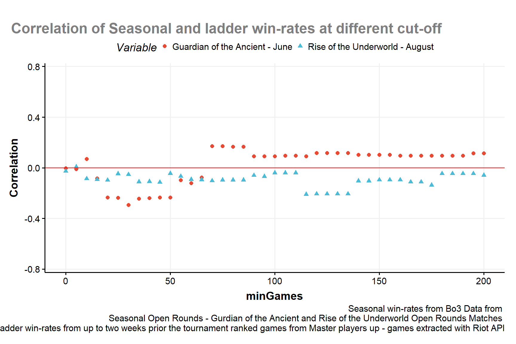
Figure 5: correlation of Seasonal Win-Rates with Ladder Win-Rates at different benchmarks of minimum amount of games for each deck
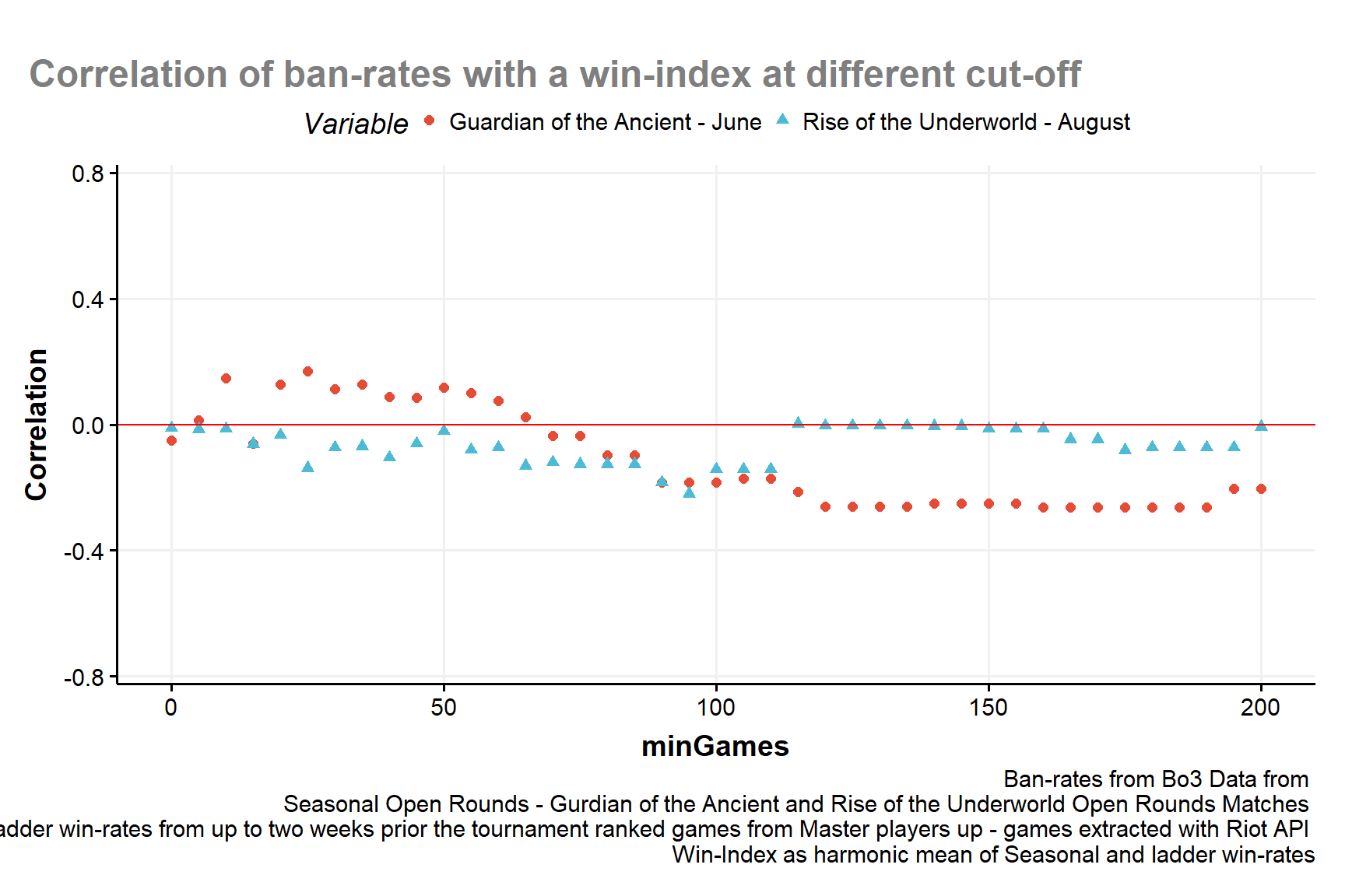
Figure 6: correlation of Ban-rates with a Win-Index computed as harmonic mean of Seasonal and ladder win-Rates with Ladder at different benchmarks of minimum amount of games for each deck
Considering the overall results the final choices to the LMI frameworks are the following:
- Having the LMI as seen in Fig:7. This is an aggregation of three subdimensions: popularity(playrate), ban and a win-subdimension which is made of the ladder and seasonal win rates. This can be justified by the correlation of the ban-index with both the play-index and the win-index. This option can
Figure 7: Possible theoretical framework for the LMI - adding both ban-rate and ladder win-rate, using three main subdimension: ban, playrate and strength
- Having the LMI as seen in Fig:8. The ban-rates shows a stronger causal relationship with the win-rates compared to the playrates (Fig:4) so considering it part of the strenght of a deck can be considered more appropriate. This the option which tries to follows the definition which was given before: ‘The performance of a deck is defined by its own strength and popularity inside the metagame.’ and is in fact the framework which is proposed.
Figure 8: Proposed LMI theoretical framework - mainteining two main subdimension and having the ban-rate as a component of the ‘strength’ subdimension
Weigths
Aggregating variable into a single index this is always done by applying weights to each component, be them equal weights or another vector. The decision can be made by following different method not all being entirely data-driven. A common way to compute the weights is by using the normalized loading factors of the first eigenvalue from the principal components. With the proposed structure both the weights for the win-index and strength index resulted in a equal weights (0.50 and 0.50). As it is both the simplest case and being confirmed by a data-driven approach equal weights are the applied weights.
Note: if we used the 3-subdimension structure the resulting weights would have been
PlayRate Index Strength Index  BanRate Index
         0.533         -0.070          0.537
Results
If we tried to apply the proposed structure for the LMI and create again the graph from the Seasonal - Rise of the Underworld report there is a clear difference from the past version. With the new framework Akshan/Sivir (DE/SH) is not in a league of its own while still being the best decks. We want to remember it is not like the previous or the current iteration is wrong and the other correct, they just measure the same/similar data in a different way. While the previous iteration created a more sensational graph we consider the current one more ‘realistic’ as the difference between Akshan/Sivir (DE/SH) and the other top performing decks was way too high. One may object that the difference is now too small but even it was the case we still consider it an improvement from the previous framework.
Conclusions
We started this article with the aim of adding the ban-rate to the LMI, contrary from out expectations this required to consider more the relationship with the selected variables and the possible causal relationship among than (in particular the ban-rates with the seasonal win-rates). To solve this problem we proposed to add a forth variable in the ladder win-rates from ranked games prior to the tournament.
A question that emerged during the analysis is about how to evaluate decks with a really small numbers of games because of an high ban-rate so if the selection filter should be adjusted to account for them. This could be done in future analysis that includes the uncertainty and sensitivity analysis.
As the new LMI doesn’t create what seems to be an outlier in Akshan/Sivir (DE/SH) a possible research question is how to determine is an even simpler way the strength of a deck. Meaning is we can translate the LMI into a tier-value, for example from ‘tier-D’ to ‘tier-S’, the commonly system used by gamers.
If we tried used the cut-off values used by Balco we would have the following results.
As the cut-off values were chosen without any particular reason behind them, a future article will try to investigate different options for the cut-off values.
To expand the application of this version of the LMI an analysis that will follow will try to apply this framework to Bo3 taken from the gauntlet and friendly Bo3.
Lastly, as the variable we are using are a result of the state of the metagame of that time future article will try to check if we can add informations regarding the quota of counter-decks for a specific deck are played in a particular time of the meta/during the tournament.
Appendix
Table 3: Quantile table
Legal bla bla
This Meta Report was created under Riot Games’ “Legal Jibber Jabber” policy using assets owned by Riot Games. Riot Games does not endorse or sponsor this project.
No official data are known at the moment of the writing. Supposition made from a series of points like the fewer amount of Master rank players when the cut-off takes place.↩︎