Introduction
Defining archetypes on Legends of Runeterra is both a simple yet complex problem. It’s simple as we can define decks for the most part by the combination of champions and regions of choice but it’s also complex by the fact that such definition is quite limited.
On our previous article/analysis we gave a possible method about how to compare archetypes and see if they can be considered from a shared common archetype or not. The method applied in that article makes use of inferential statistical analysis to reach a conclusion. Sadly, it’s also a methodology that’s more fitting a posterior analysis, when hypothetical archetypes are already defined, a tool more fitted to refine the results and not to define archetypes.
To identify archetypes, a more fitting methodology is a form of exploratory data analysis (EDA) known as Clustering Analysis (CA). Its aim is to find subgroups (or clusters) in our data without relying on a response variable, also why it’s called unsupervised learning.
As useful as it is CA suffer from a fundamental problem of not being able to check out the quality of the results. With a vast array of different algorithms and hyper-parameters this also means that finding the the “correct” way to use a CA to define archetypes (which was supposed to be the aim of this article) is not only impossible, it’s also seeing the CA in the wrong way. Surely some choices are better than others but there is no perfect answer and to be fair, this was making us, was making me, procrastinating the writing of this article. The result, or maybe compromise was to reduce the scale on this article which will be a small dive into the cluster analysis. While I want to provide some food for thought to others in the end the main recipient of the article is myself, to provide me a more solid foundation on the topic and how to approach it, knowing the basic limitations of what I’m planning to use.
Clustering
Clustering is an heterogeneous domain. Applied in a wide range of disciplines with the aim of finding subgroups or clusters, in a data set.
Clustering is considered a basic tools of data mining along side the supervised learning domain (clustering is defined as unsupervised learning) but differently from it clustering suffers from a lack of theoretical understanding of its application.
Each example, even the most basic face the problem of selecting which algorithm to apply (known as “the user dilemma”); there is no principled method to guide the selection. While the theory is starting to identify differences between clustering methods, this field is still in it’s early phase and the applications are left to ad hoc decisions. If decisions are being made usually they are defined by engineering properties as run times or memory used.
This is also a consequence of clustering being a problem not well defined. As statistics is all about the question, it’s not possible to define the ‘correct’ clustering if we have no definition of what it is correct.
Of course, to make this concrete, we must define what it means for two or more observations to be similar or different. As a general rule of rule of thumb we try to aggregate similar observations in the same group while making it so that the differences between groups is overall high.
K-Means
K-Means clustering is a commonly used approach; it’s simple yet performing method for partitioning a data set into K distinct, non-overlapping clusters. The K-Means algorithm has as hyper-parameter the numbers of desired number of clusters K, from that the algorithm will try to create the best k-clusters based by an optimization function. To start, there is an initialization step that randomly assign one of the k cluster to each data point, then, the algorithm iterates until cluster assignments stop changing:
For each of the K clusters, compute the cluster centroid or barycentre.
Assign each observation to the cluster whose centroid is closest (where closest is defined using Euclidean distance)
As mentioned, the number of clusters that will be returned is a pre-condition to perform K-Means. The problem of selecting K is far from simple.
This issue, along with other practical considerations that arise performing K-Means clustering like: should variables should be first be standardized in some way?1
There are some general guides about how to choose the optimal number of clusters.
The most commonly used rules are:
Elbow method
As the K-Means clustering tries to define clusters such that the total intra-cluster variation (known as total within-cluster variation or total within-cluster sum of square) is minimized
\(minimize(\sum_{k=1}^KW(C_k))\)
The total within-cluster sum of squares (wss) measures the compactness of the clustering; we want it to be as small as possible so we can use its value in function of k (number of clusters) and plot them.
The location of a knee/elbow in the plot is generally considered as an indicator of the appropriate number of clusters.
This is because normally the wss is related to the number of cluster by a monotone decreasing function, meaning that if the aim is simply to minimise wss then having k = n clusters each of them corresponding to a single element which would give the minimum wss.2
One must search the optimal value we are searching for is in \(1 < k < |X|\) finding a compromise between the reduction of the objective function wss and the dimension of the hyper-parameter k.
Common practise is to use the Elbow method as it tells us when increasing k is less “worth” compared to the reduction in wss.
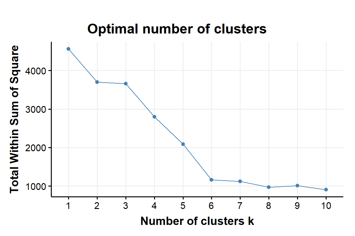
Figure 1: within sum of squares as a fnction of number of clusters obtained with K-Means applyed to the example data set
Silhouette method
Prior to this article I’m not sure I even heard about this value: From Wikipedia, the silhouette is defined as:
The silhouette value is a measure of how similar an object is to its own cluster (cohesion) compared to other clusters (separation). The silhouette ranges from −1 to +1, where a high value indicates that the object is well matched to its own cluster and poorly matched to neighboring clusters. If most objects have a high value, then the clustering configuration is appropriate. If many points have a low or negative value, then the clustering configuration may have too many or too few clusters.
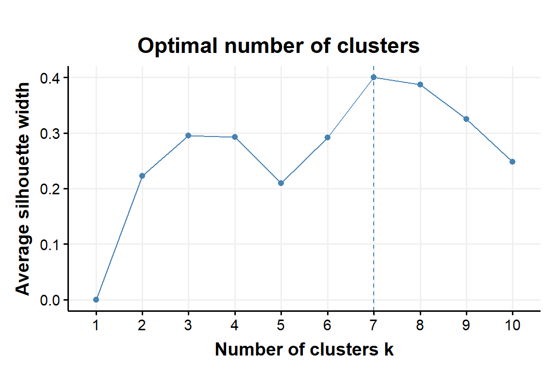
Figure 2: Silhouette as a fnction of number of clusters obtained with K-Means applyed to the example data set
Fig:1 and Fig:2 show the results from the described methods. Using K-Means the algorithm is suggesting a number of k clusters with k around 6 or 7. We will discuss later the quality of these choices, for now we will focus on the algorithm per se.
K-Means while a powerful tool in many fields doesn’t seems to be the best choice for the archetype problem. Its main con is it requires the user to define a priori the number of clusters it needs to find.
This is almost the opposite of what we would like from the algorithm that should aid us in defining archetypes. Ideally we would prefer if the clustering methods gives us some indications regarding which decks to aggregate into a single archetype, or even division of sub-archetypes if the region+champion combination is not enough to distinguish archetypes. In addition, K-Means presents other problems like having to start with a randomized assignment of clusters, of course this can be controlled by having fixed seeds; it’s also common practises to repeat K-Means multiple times in order to find the ‘mean’-cluster assignment. Yet, the methods is overall quite sensitive to noise/outliers. Even the methods that should help us can be quite subjective, if n is very large defining the location of the knee can be not as clear as in this example.
Lastly but not less important, differently from other class of cluster algorithm, there is less flexibility regarding the measure/distance to compare decks.
Hierarchical Clustering
One potential disadvantage of K-Means clustering is that it requires us to pre-specify the number of clusters K. Hierarchical clustering is an alternative approach which does not require that we commit to a particular choice of K. Hierarchical clustering has an added advantage over K-Means clustering in that it results in an attractive tree-based representation of the observations, called a dendogram.
The hierarchical clustering dendogram is obtained via an extremely simple algorithm. We begin by defining some sort of dissimilarity measure between each pair of observations. Most often, Euclidean distance is used and the algorithm proceeds iteratively. Starting out at the bottom of the dendogram, each of the n observations is treated as its own cluster. The two clusters that are most similar to each other are then fused so that there are now n-1 clusters. The algorithm proceeds in this fashion until all of the observations belong to one single cluster, and the dendogram is complete.
This algorithm seems simple enough, but one issue has not been addressed. Consider the aggregation step, how do we determine which cluster should be fused with another cluster? We have a concept of the dissimilarity between pairs of observations, but how do we define the dissimilarity between two clusters if one or both of the clusters contains multiple observations? The concept of dissimilarity between a pair of observations needs to be extended to a pair of groups of groups of observations. This extensions is archived by developing the notion of linkage, which defines the dissimilarity between two groups of observations.
The five most common types of linkage are:
- Single Linkage: The distance between two clusters is the minimum distance between any single data point from the first cluster with any single data point from the second cluster.
With d as a distance function
\[\begin{equation} \textit{l}_{SL}=min_{a\in A,b\in B}d(a,b) \tag{1} \end{equation}\]By applying Single linkage to the example data set the resulting dendogram is:
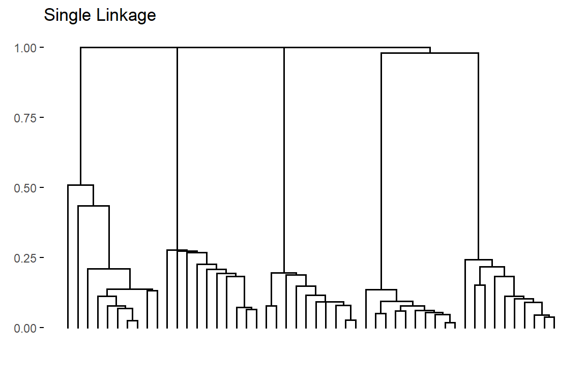
Figure 3: Dendogram obtained by applying Single linkage to the example data set
From Fig:3 it’s possible to notice how Single linkage can result in extended, trailing clusters in which single observations are fused one-at-a-time.
- Complete Linkage: The distance between two clusters is the maximum distance between any single data point from the first cluster with any single data point from the second cluster.
By applying Complete linkage to the example data set the resulting dendogram is:
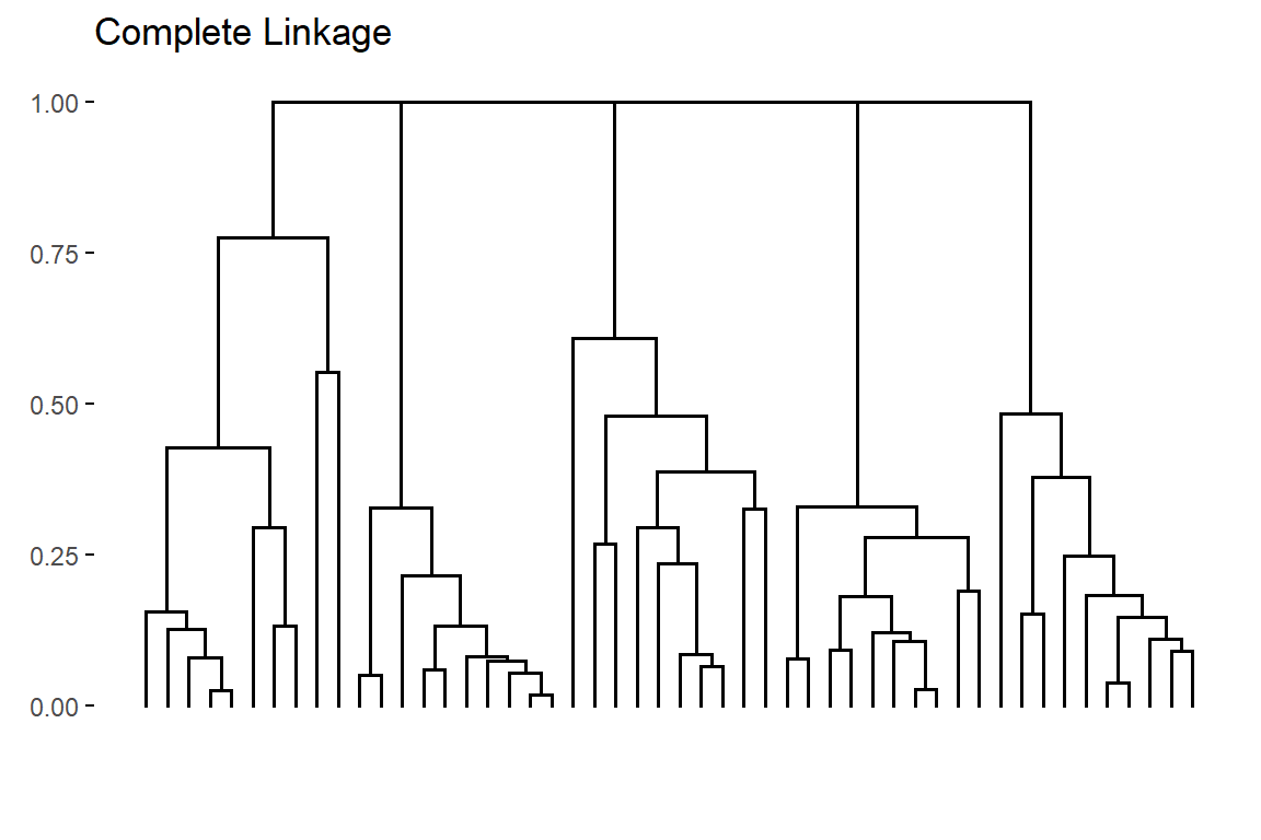
Figure 4: Dendogram obtained by applying Complete linkage to the example data set
Clusters resulting from Complete linkage tend to have a spherical structure and are usually more compact.
- Average Linkage: The distance between two clusters is the average distance between any single data point from the first cluster with any single data point from the second cluster.
By applying Average linkage to the example data set the resulting dendogram is:
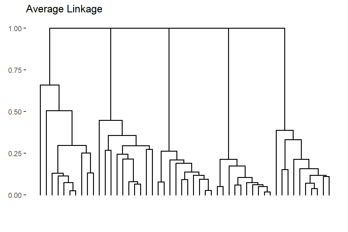
Figure 5: Dendogram obtained by applying Average linkage to the example data set
As intuitively as it is, clusters resulting from Average linkage is a less “extreme” version of both Single and Complete linkage
- Centroid Linkage: The distance between two clusters is the distance between the two centroids/barycentre that are defined from the data points within respectively the first and second cluster.
Centroid linkage can result in undesirable inversions, whereby two clusters are fused at a height below either of the individual clusters in the dendogram.
\[\begin{equation} \textit{l}_{Centroid}(A,B,d)= d(\overline{x},\overline{y}) \tag{4} \end{equation}\]By applying Average linkage to the example data set the resulting dendogram is:
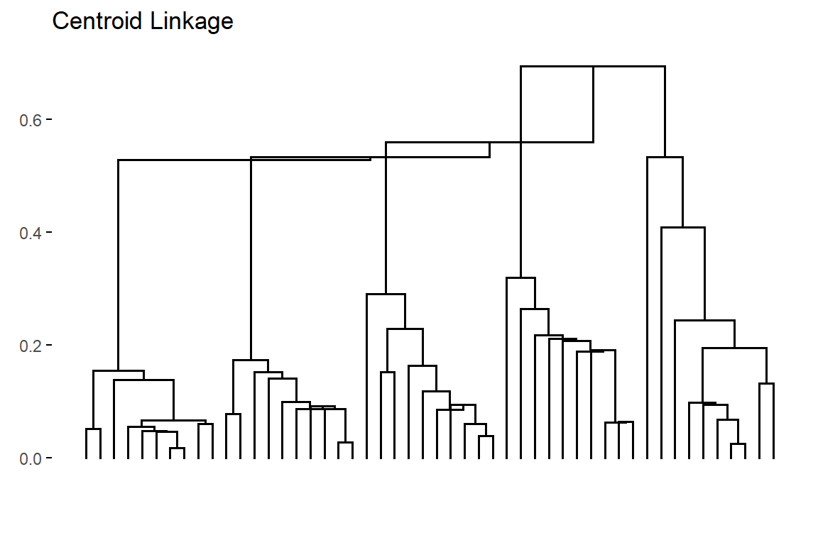
Figure 6: Dendogram obtained by applying Centroid linkage to the example data set
From Fig:6 it’s possible to notice the inversion phenomenon that can occurs with Centroid linkage with as the clusters are fused at a height below either of the individuals clusters in the dendogram.
- Ward’s Method: This method does not directly define a measure of distance between two points or clusters. It is an ANOVA based approach. One-way univariate ANOVAs are done for each variable with groups defined by the clusters at the stage of the process. At each stage, two clusters merge that provide the smallest increase in the combined error sum of squares. (We won’t try this method)
The choice of number of clusters with hierarchical clusters can be done the same way we did with K-Means (like wss or silhouette). A strength of hierarchical clustering is making the choice of k by being guided by the dendogram.
The height of the fusion, provided on the vertical axis, indicates the (dis)similarity between two observations. The higher the height of the fusion, the less similar the observations are.
Similarly it’s possible to cut the dendogram and define k clusters. The height of the cut to the dendogram controls the number of clusters obtained. It plays the same role as the k in K-Means clustering. In order to identify sub-groups (i.e. clusters).
From all the dendograms there is evidence that suggest choosing around 5 or 6 clusters is the optimal choice. Again, we will discuss later the ‘quality’ of this choice.
Defining the problem
Upping the game
Up until now what has being described is the basic of the basic on clustering which could be found in any article/guide/course on the subject. What will follows is more akin as a self-explanation of points that could be worth to evaluate in order to approach the algorithm problem. Additional algorithms will be introduced with both their pros and cons. After describing all the applied algorithms we will at last explain the example used in this article to highlight what seems to be more interesting to explore for future analysis in the search of a way to define archetypes.
Let us introduce a couple of point from a discussion with Drisoth and their effects:
The point of clustering is to increase sample size by being able to talk about a large section of decks in aggregate rather than each one individually. (Auhor Note: so using the existing data from played games) With that goal in mind, clustering off-meta decks with low sample size as noise is not a large loss of information, since even if we clustered similar decks together the cluster would still have too little data for any meaningful analysis to be done on it.
From this approach three questions comes to mind:
Should there exist outliers that’s best not to assign to a cluster?
If the question is formulated simply like that, with no other conditions, then yes, there is no deny that outliers and/or noise exists in the archetype problem and the best way to deal with them would be not assigning them to clusters.
The reason is obvious: it’s possible for a random pile of 40 cards to resemble an archetype, but, for the most cases it would likely turn into just that, a random pile of cards.
Their existence is certain, even worse many cluster algorithm are sensitive to noise and outliers and at various degree so are the methods described up until know. If K-Means starts on an outlier it won’t be easily dealt with, also a reason why it’s best practise to repeat K-Means several times to avoid being too depending on the original random choice at the initialization step. In (Agglomerative) Hierarchical Clustering (AHC), if an outlier is wrongly assigned to a cluster this error will be propagated on all the following steps with no way to intervene.3
Among the class of clustering algorithms that are able to deal with outliers and noise DBSCAN is probably the most popular and cited. The algorithm will be explained in the following paragraph.
Should the data be weighted?
While being developed only recently, the concept of a weighted clustering framework can be traced back into the ’70. A more formal definition has has been developed while also introducing a series of mathematical properties related to the weights (Ackerman et al. 2016). The use of weights can be seen as a more generalized definition of centroid if not even just its description as barycentre also called centre of mass.
It is easy to see that using unweighed data can be seen as having the same weight 1 on all data. Applying weight would be the same as having duplicates as multiple points with mass would correspond to a single point with weight equal to the sum of masses. Similarly a point of zero mass can be seen as non-existent. From this, for many algorithms the consequence would be such as: instead of starting the iterative steps from the leafs, they would start from point-clusters of different masses.
Following the definition of weighted clustering, one may ask what effect does this have on the clustering algorithms? (Ackerman et al. 2016) introduced the properties related to the response to weighted data
Be it \((X,d)\) a dissimilarity function and \(|range(A(X,d,k))|\) the range of a partitional algorithm on a data set defined as the number of clusterings it outputs on that data over all weights functions:
Weight Robust Algorithm A partitional algorithm \(A\) is weight-robust if for (X,d) and \(1 < k < |X|\) \(|range(A(X,d,k))|=1\). This means that the output of a weight robust algorithm is unaffected by the choice of weights
Weight Sensitive Algorithm A partitional algorithm \(A\) is weight-sensitive if for (X,d) and \(1 < k < |X|\) \(|range(A(X,d,k))|>1\). This case imply that no matter the original data, the result can be changed in response of the use of weights. Even if we would like to use weights to guide our output this properties doesn’t seems desirables as we may want to not be too subjected to the weights. Of course it’s not like we can’t have the same results when applying different weights if the geometry of out data helps us. Yet, no matter the case we can’t be sure that the algorithm won’t be affected by the weights.
Weight Considering Algorithm A partitional algorithm \(A\) is weight-considering if
- \(\exists\) (X,d) and \(1 < k < |X|\) so that \(|range(A(X,d,k))| = 1\) and
- \(\exists\) (X,d) and \(1 < k < |X|\) so that \(|range(A(X,d,k))| > 1\)
We took this detour of explaining how an algorithm can react to the addition of weights as we needed to point out that in some cases their inclusion doesn’t bring any difference to the results.
Also, while what we described was defined around duplicated (or weighted) data, this also apply to near-duplicated data.
In addition these properties can tell us a bit more of the algorithm in question.
The next figure gives an idea of what to expect for robust and sensitive cases.
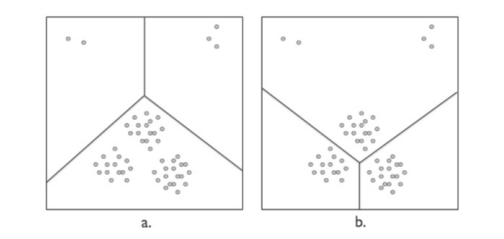
We must remind how there is not correct partitioning, it all depends by the characteristics of each case study.
What this example wants to convey is that if we know something of the underlying geometry of our data, and, what we would like our algorithm to favour, while there is no correct clustering we can still reduce a little “the user’s dilemma” of which algorithm to choose from.
Among the algorithms showed up until know Single linkage and Complete linkage are weight robust (and not many others more generally possess this property). Fig:7 shows an example with Single linkage
Ward and K-Means (as many other variant of the ‘k-family’) are weight sensitive and Average linkage is weight considering. Fig:8 shows an example with Average linkage. While only marginal, we can see the effect of applying weights on the second ‘main’ cluster.
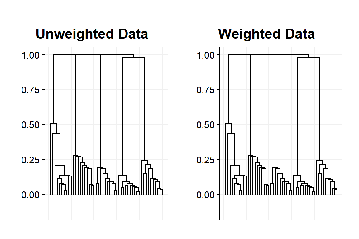
Figure 7: Dendogram obtained with unweighted and weighted using Single linkage with the example data set
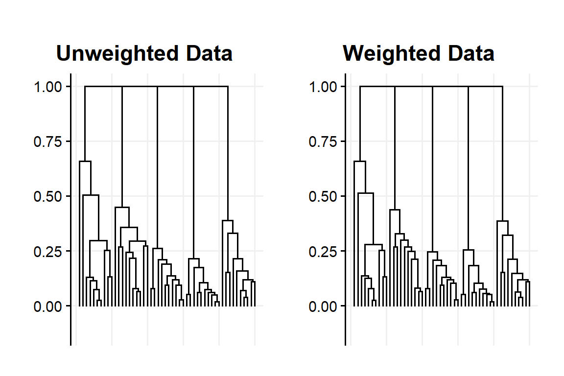
Figure 8: Dendogram obtained with unweighted and weighted using Average linkage with the example data set
So remember kids, don’t try weighted data when applying Single-linkage at home (it’s useless)
| Partional | Hiercarchical | |
|---|---|---|
| Weight Sensitive | K-Means, k-medoids,k-median, Min-sum | Ward's Method, Bisecting K-Means |
| Weight Considering | Ratio-cut | Average Linkage |
| Weight Robust | Min-diameter, k-center | Single/Complete Linkage |
| A classification of clustering algorithms based on their response to weighted data. Source: Ackerman2016 | ||
Is there any other way to use the metagame data?
This question is more a result of seeing the Drisoth philosophy in a different way. Just because we want to be guided by the metagame in order to define archetypes doesn’t mean the weighting of data is the only option.
From out perspective if we want to use the games data the reason is because we have a clear idea about what to expect from certain decks. From games we have an idea of what can identify a specific archetype, sometimes we may even have what is an ideal deck-list, a deck-list that is exemplar.
The easiest way to introduce this concept is by describing how it’s possible to use it starting from the K-Means algorithm.
In K-Means a cluster’s centre is defined by the centroid obtained from its points, aside for this they have no constraints about their position in the data space.
If we add the constraint that the centre must an actual data point the ‘centre’ is called examplars. The algorithm that can be defined by this change in K-Means is called K-medoids.
K-Medoids only slightly differ from K-Means as:
Instead of just computing the cluster’s centroid we find the existing data point whose average dissimilarity between it and all other members of the cluster is minimal.
We can use any distance to find the examplar.
An even more interesting approach is applied by a message-based cluster algorithm called Affinity Propagation.
What is interesting about these methods is that they associate a real data point to each cluster. This open for a variety of decisions and quality-check options like being able to evaluate the quality of the identified clusters, checking the similarity within-cluster or differences between-clusters with a reduced number of points/references.
As it is more complex compared to K-Medoids, Affinity Propagation will be described in the next paragraph after DBSCAN.
DBSCAN
DBSCAN (Density-Based Spatial Clustering of Applications with Noise) is a fairly recent algorithm as it was introduced in 1996 and it’s currently the most popular density-based method.
DBSCAN uses two hyper-parameters to define the clusters:
minPts: for a region to be considered dense, the minimum number of points required are minPts
eps: to locate data points in the neighbourhood of any points, eps \(\epsilon\) is used a distance measure.
From these parameters two concept are also introduced: Density Reachability and Density Connectivity
Reachability: in terms of density, establishes a point to be reachable from another if it lies within a particular distance \(\epsilon\) from it. This property is not symmetrical
Connectivity: on the other hand involves a transitivity based chaining-approach to determine whether points are located in a particular cluster.
This algorithms and concepts are based on the idea that clusters are defined by dense data space, dense with points and with other clusters being separated by region of low density.
This type of clustering algorithm connects data points that satisfy particular density criteria (minimum number of objects within a radius). After DBSCAN clustering is complete, there are three types of points: core,border,and noise.
Core: is a point that has some (minPts) points within a particular \(\epsilon\) distance from itself.
Border: is a point that has at least one core point at distance \(\epsilon\).
Noise: is a point that is nether border nor core. Data points in sparse area required to separate clusters are considered noise and broader points.
The algorithm proceeds as it follows:
DBSCAN starts with a random data point (not-visited). Note: even if this step is randomized the algorithm is almost heuristic and robust to the initial choice.
The neighbourhood of this point is extracted using a distance \(\epsilon\)
If there are sufficient data points within this area the current data point becomes the first point in the newest cluster, else, the point is marked as noise and visited.
The point within its \(\epsilon\) distance neighbourhood also became a part of the same cluster for the first point in the new cluster. For all the new data points added to the cluster above, the procedure for making all the data points belong to the same cluster is repeated.
The above two steps are repeated until all points in the cluster are determined. All points within the \(\epsilon\) neighbourhood of the cluster have been visited and labelled. Once we’re done with the current cluster, a new unvisited point is retrieved and processed, leading to further discovery of the cluster or noise. The procedure is repeated until all the data points are marked as visited.
Usually to find the the value for \(\epsilon\) we use the a plot of the k-nearest neighbour (kNN) distances for the dataset with all the distances being plotted from the smallest to largest.
In R, for the package ‘dbscan’ the heuristic method to find \(\epsilon\) is a follows:
A suitable neighborhood size parameter eps given a fixed value for minPts can be found visually by inspecting the kNNdistplot of the data using k = minPts -1 (minPts includes the point itself, while the k-nearest neighbors distance does not). The k-nearest neighbor distance plot sorts all data points by their k-nearest neighbor distance. A sudden increase of the kNN distance (a knee) indicates that the points to the right are most likely outliers. Choose eps for DBSCAN where the knee is.
Since the example data set data is quite small we will assign minPts=2 and so using k=1
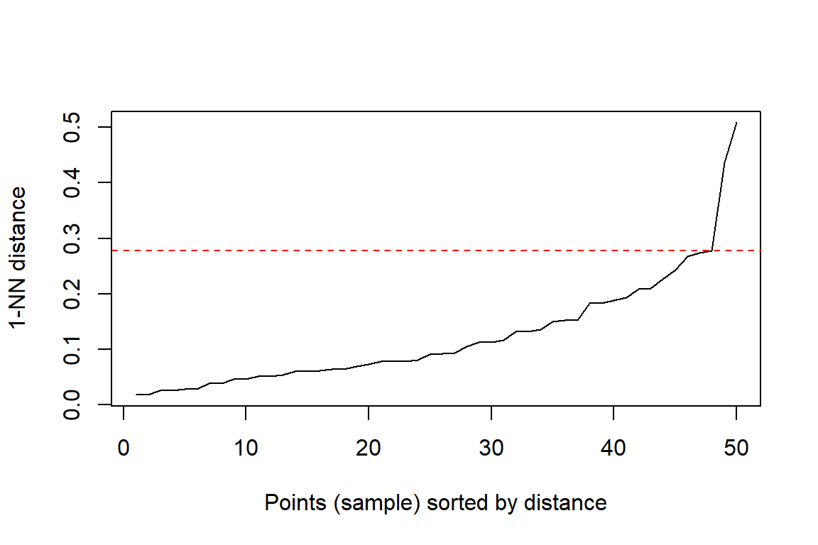
We will do the clustering with \(\epsilon\)=0.2775 and using both the cosine similarity.
In addition we will replicate a previously used methodology by Drisoth by choosing the Manhattan distance and \(\epsilon\)=37 (40-3 ‘cards’ similarity)4
When applied to the example data set we get:
DBSCAN clustering for 50 objects.
Parameters: eps = 0.2775, minPts = 2
The clustering contains 5 cluster(s) and 2 noise points.

 0  1  2  3  4  5
 2 10 10 10 10  8

Available fields: cluster, eps, minPts
DBSCAN with the cosine similarity, \(\epsilon\)=0.2775 and minPts=2 return 5 cluster with 2 noise points
DBSCAN clustering for 50 objects.
Parameters: eps = 37, minPts = 2
The clustering contains 5 cluster(s) and 1 noise points.

 0  1  2  3  4  5
 1 10 10 10 10  9

Available fields: cluster, eps, minPts
DBSCAN with the Manhattan distance, \(\epsilon\)=0.2775 and minPts=2 returns again 5 clusters but only 1 noise point
Does DBSCAN scale well?
In this article we introduced the problem of a lack of consideration of a clustering properties in order to decide which clustering algorithm to apply to our data set.
A series of weight-related properties were introduced to make us aware how some algorithms can be influenced or not by weighted data.
More generally it’s possible to define a wide series of clustering methods properties Ackerman and Ben-David (2011). Among them there is property that we believe should be present for any clustering methods we are planning to use for the archetype problem: Locality
\(\forall\) domain (X,d) and number clusters, k, if X’ is the union of k’ clusters in F(X,d,k) for some k’ \(\leq\) k then, applying F to (X’,d) and asking for a k’-clustering, will yield the same clusters that started with
It is pretty clear why we wants this property. It we cluster a subset of an archetype, we should still get the a result consistent with the same archetype.
We wondered if this property is satisfied by DBSCAN because of the minPts hyper-parameter and if its value would be able to determine different results with the same setting.
We can say that DBSCAN satisfy this property. This is easily proved by the existence of the DBSCAN extension HDBSCAN which convert DBSCAN into an hierarchical algorithm. Because of HDBSCAN we can then use the following lemma introduced by Ackerman (Ackerman and Ben-David 2011):
What is the linkage method applied by DBSCAN? Simple-linkage. In fact, DBSCAN search the the minPts at a \(\epsilon\) distance which is a more constrained use of single-linkage.
We can also point that locality specify that the sub-set in made of k’ clusters so it exclude the choice of picking a subset of a mixture of noise points and a partial subset of a cluster. Because of this we know that the cluster will satisfy again the definition of cluster by DBSCAN allowing locality to be satisfied.
TLDR: DBSCAN is a fine good as an algorithm to define archetypes. It may have other reasons to make us not completely sure about using this algorithm but this key property is satisfied.
K-Medoids (results)
We report the results in seeking the optimal number of clusters using K-Medoid using two different metric, the Manhattan distance (or L1 distance) and the Cosine similarity to the example data set.
As with the other methods the results will be discussed at the end of the article.
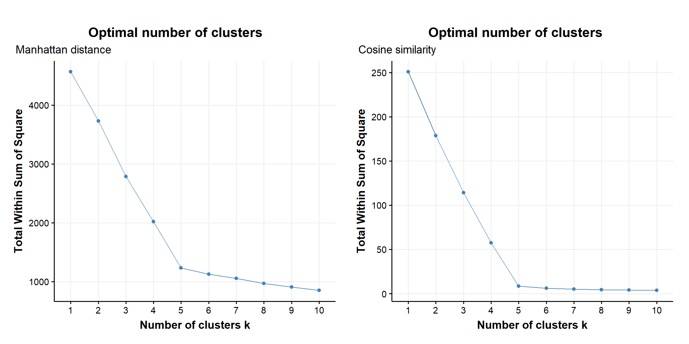
Figure 9: within sum of squares as a fnction of number of clusters obtained with K-medoids and manhattan & cosine metric applyed to the example data set
Affinity Propagation Clustering
Affinity Propagation Clustering (APcluster) is a fairly recently introduced clustering methods Frey and Dueck (2007).
It is based on the passage of messages between data points to detect patterns in data.
As K-Medoids it uses examplars data point.
Two messages are exchanged between data points:
Responsibility r(i,k) is sent from i to k and correspond to the accumulated evidence for how well-suited k is to server as the examplar for i, taking into account other potential exemplars for point i
Availability a(i,k) is sent from k to i and correspond to the accumulated evidence for how appropriate it is for i to choose k as its examplar, taking into account the support from other points that point k should be examplar
The iteration steps updates the following values:
\(R(i,k) \leftarrow S(i,k) - max_{k' \neq k}(A(i,k')+S(i,k'))\)
\(A(i,k) \leftarrow min{(0,R(k,k')+\sum_{j \notin {i,k}}max(0,R(j,k) ) )}\)
\(A(k,k) \leftarrow max_{j \neq k}(0,R(j,k))\)
The examplar are chosen as the point from whom responsibility+availability for themselves is positive \(r(i,i)+a(i,i)>0\)
S(i,k) is the similarity matrix we provide which doesn’t even need to satisfy the usual metric property, not only it doesn’t have to satisfy the triangular inequality but it doesn’t even need to be symmetric.
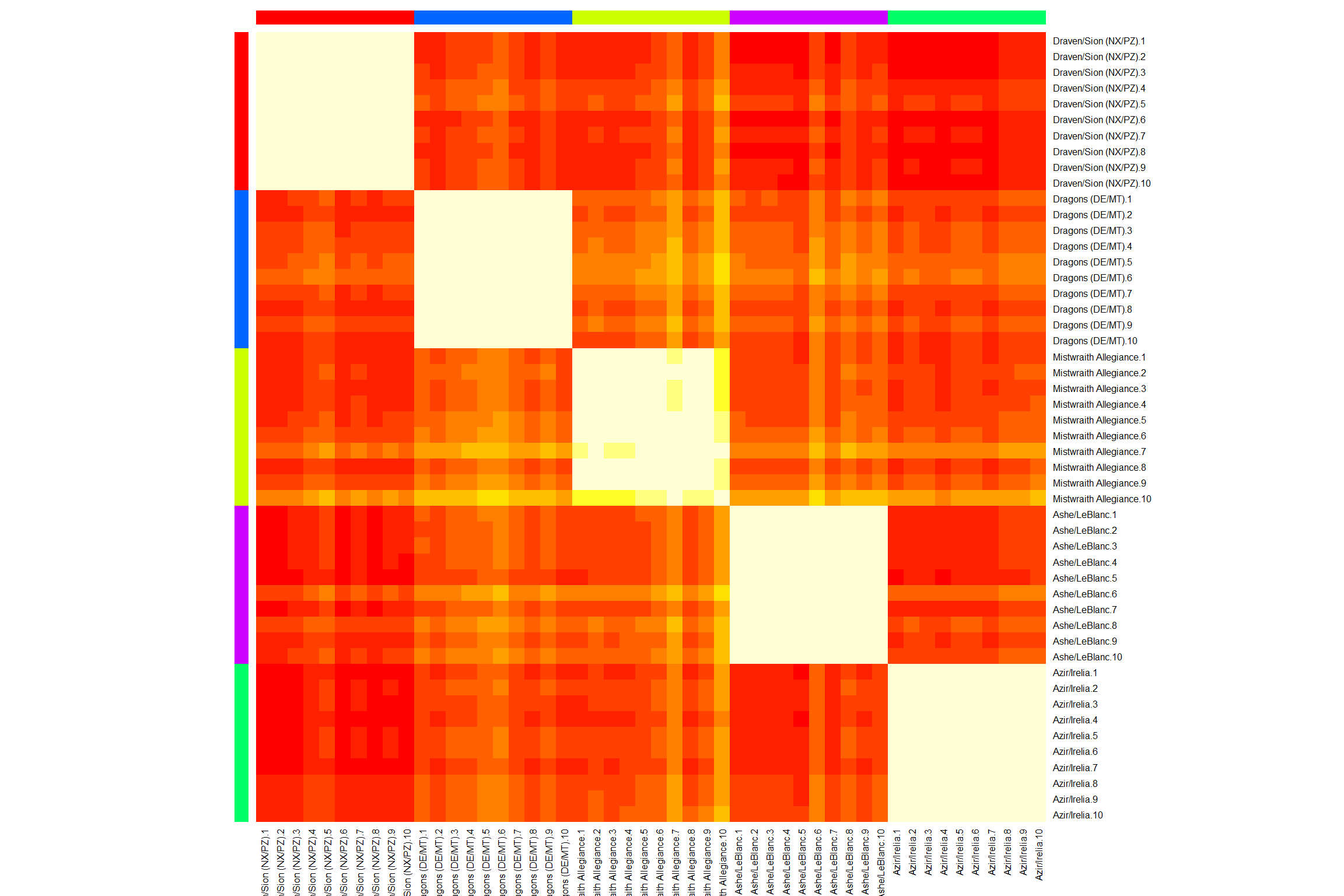
In this example we will use the similarity matrix provided by the application of the cosine similarity. What follows in the heatmap obtained by applying APcluster to the example data set.
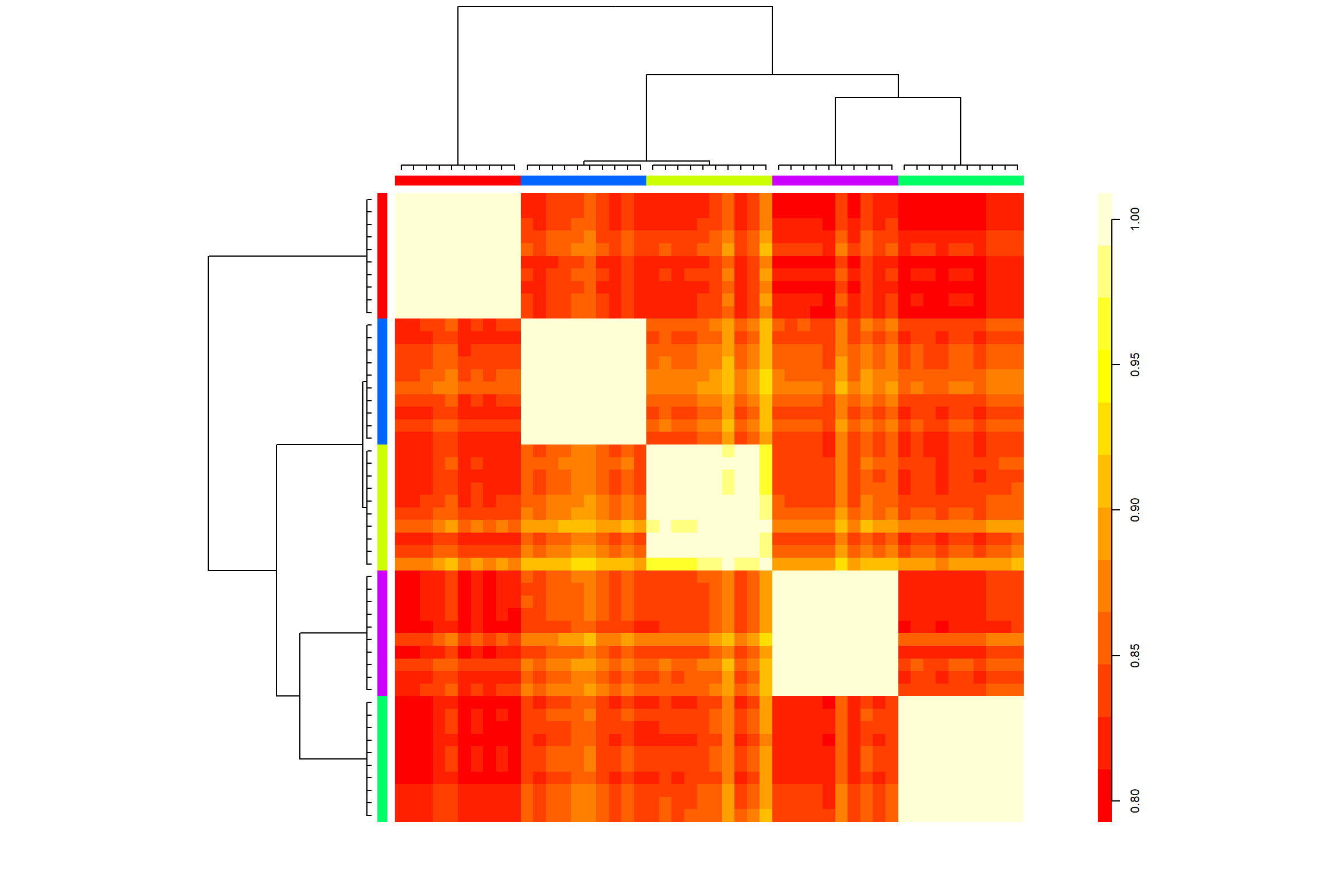
Figure 10: Heatmap obtained by applying APcluster to the example data set
Similarly to most of the other methods, the algorithm is suggesting us the presence of 5 archetypes with one of them being a little less homogeneous compared to the other 4.
As we finally showed all the algorithm we planned to introduce and explain, we can finally describe the data set used an show more in the detail the results we had.
Data
The example used in this article is made out of 50 decks.
Five archetypes with different regions & different play style have been selected as ‘core’
- Ashe/LeBlanc
- Azir/Irelia
- Dragons (DE/MT)
- Draven/Sion (NX/PZ)
- Mistwraith Alligiance
Does this mean that the correct answer of k-cluster we should have expected was 5? Well… not necessarily, there is in fact a catch that I didn’t mention. Among the ‘archetypes’ I also selected some of their sub-archetypes.
To help explain what I actually choose I’ll also report the code I used to sample the deck-lists.
# how I selected the decks, it is reproducible as more decks will be inserted in the DB

#' archetypes names
archetypes <- c(
  "Ashe/LeBlanc",           # 75/25 noMarauder/Marauder
  "Azir/Irelia",            # 100
  "Dragons (DE/MT)",        # 30/70 J4/PureDrake "Aurelion Sol/Jarvan IV/Shyvana",  "Aurelion Sol/Shyvana",
  "Draven/Sion (NX/PZ)",    # 80/20 DravenSion/RubinBait
  "Mistwraith Allegiance"   # 50/50 Targon/Piltover
)

#' sampling a bigger number of decks for a bigger example I ended up not using
set.seed(123)
Rep1 <- LoR.Deck.RMD |>
  filter( archetype == "Ashe/LeBlanc" & is.na(archetype_pretty) ) |>
  slice_sample(n = 75) |>
  pull(deck_code)

set.seed(123)
Rep2 <- LoR.Deck.RMD |>
  filter( archetype_pretty == "Marauder" ) |>
  slice_sample(n = 25) |>
  pull(deck_code)

set.seed(123)
AI <- LoR.Deck.RMD |>
  filter( archetype == "Azir/Irelia", ) |>
  slice_sample(n = 100) |>
  pull(deck_code)

set.seed(123)
Dragon1 <- LoR.Deck.RMD |>
  filter( archetype == "Aurelion Sol/Jarvan IV/Shyvana" ) |>
  slice_sample(n = 30) |>
  pull(deck_code)

set.seed(123)
Dragon2 <- LoR.Deck.RMD |>
  filter( archetype == "Aurelion Sol/Shyvana" ) |>
  slice_sample(n = 70) |>
  pull(deck_code)

set.seed(123)
Sion1 <- LoR.Deck.RMD |>
  filter( archetype == "Draven/Sion (NX/PZ)" & is.na(archetype_pretty) ) |>
  slice_sample(n = 80) |>
  pull(deck_code)

set.seed(123)
Sion2 <- LoR.Deck.RMD |>
  filter( archetype_pretty == "RubinBait - Draven/Sion", ) |>
  slice_sample(n = 20) |>
  pull(deck_code)

set.seed(123)
Mist1 <- LoR.Deck.RMD |>
  filter( archetype_pretty == "Mistwraith Allegiance" & str_detect(factions,"Targon") ) |>
  slice_sample(n = 50) |>
  pull(deck_code)

set.seed(123)
Mist2 <- LoR.Deck.RMD |>
  filter( archetype_pretty == "Mistwraith Allegiance" & str_detect(factions,"Piltover") ) |>
  slice_sample(n = 50) |>
  pull(deck_code)

#' sub-sampling the decks I ended up not using
LoR.Archetype.Ex <- rbind(
  LoR.Deck.RMD[ deck_code %in% Rep1, ],
  LoR.Deck.RMD[ deck_code %in% Rep2, ],
  LoR.Deck.RMD[ deck_code %in% AI, ],
  LoR.Deck.RMD[ deck_code %in% Dragon1, ],
  LoR.Deck.RMD[ deck_code %in% Dragon2, ],
  LoR.Deck.RMD[ deck_code %in% Sion1, ],
  LoR.Deck.RMD[ deck_code %in% Sion2, ],
  LoR.Deck.RMD[ deck_code %in% Mist1, ],
  LoR.Deck.RMD[ deck_code %in% Mist2, ]
)

mini.ex <- c(Rep1[1:7], # Ashe/LB
             Rep2[1:3], # Marauder
             AI[1:10],  # AI
             Dragon1[1:3], # with J4
             Dragon2[1:7], # no J4
             Sion1[1:8],   # OG
             Sion2[1:2],   # fake-burn
             Mist1[1:5],   # MT
             Mist2[1:5])   # PnZ
So if I had to better specify what the sample contains:
Five archetypes with different regions & different play style have been selected as ‘core.’ Almost all archetypes contains some variants of the same decks
- Ashe/LeBlanc
- 7 decks of ‘standard’ Ashe/LB
- 3 decks of the ‘Marauder’ variant which is defined by playing 3 copies of Strength in Numbers in a Freljord/Noxus deck. No Ashe/LB could be sampled from this subgroup
- Azir/Irelia
- 10 decks of Azir/Irelia
- Dragons (DE/MT)
- 3 decks with at least Jarvan IV/Shyvana/Aureion Sol
- 7 decks with at least Shyvana/Aureion Sol (but no Jarvan IV)
- Draven/Sion (NX/PZ)
- 8 decks of ‘standard’ Draven/Sion
- 2 decks of the Rubin-Bait variant
- Mistwraith Alligiance - Mistwraith Alligiance decks are defined by having 3 copies Mistwraith and overall 37 SI cards
- 5 decks of a Mistwraith decks with Mount Targon and 3 copies of Pale Cascade
- 5 decks of a Mistwraith decks with PnZ and 3 copies of Iterative Improvements
Something that I want to highlight of the Mistwraith decks is that the option for the champions of choice was completely free. In this archetype after all the champions plays a marginal role to the deck’s strategy. The following table shows the champions combination’s distribution.
| archetype | n | percent |
|---|---|---|
| Elise/Kalista (MT/SI) | 4 | 0.4 |
| Elise/Kalista (PZ/SI) | 2 | 0.2 |
| Kalista (PZ/SI) | 2 | 0.2 |
| Kalista/Nocturne (MT/SI) | 1 | 0.1 |
| Viego (PZ/SI) | 1 | 0.1 |
The Mistwraith example could be said it was key for why and how I want to approach the archetype problem. SI is probably the region who is less tied by its champions per se. Thresh is more an exception but for example Kallista and Elise are included in a wide variety of decks that cannot be identified simply by their use.
In addition to the ‘champions problem’ the Mistwraith has the additional problem of being the first archetype to this is not bound by the regions it use. As of now Bandle expanded this concept with a variety of BandleTree Decks, but Mistwraith was the OG case.
Resuls
K-Means
| 1 | 2 | 3 | 4 | 5 | |
|---|---|---|---|---|---|
| Ashe/LeBlanc | 0 | 0 | 0 | 7 | 0 |
| Azir/Irelia | 0 | 0 | 0 | 0 | 10 |
| Dragons | 0 | 7 | 0 | 0 | 0 |
| Dragons+J4 | 0 | 3 | 0 | 0 | 0 |
| Draven/Sion | 8 | 0 | 0 | 0 | 0 |
| Marauder | 0 | 0 | 0 | 3 | 0 |
| Mistwraith(MT) | 0 | 0 | 5 | 0 | 0 |
| Mistwraith(PnZ) | 0 | 0 | 5 | 0 | 0 |
| RubinBait-Sion | 2 | 0 | 0 | 0 | 0 |
| 1 | 2 | 3 | 4 | 5 | 6 | 7 | |
|---|---|---|---|---|---|---|---|
| Ashe/LeBlanc | 0 | 0 | 0 | 0 | 0 | 7 | 0 |
| Azir/Irelia | 0 | 0 | 0 | 0 | 10 | 0 | 0 |
| Dragons | 0 | 7 | 0 | 0 | 0 | 0 | 0 |
| Dragons+J4 | 0 | 3 | 0 | 0 | 0 | 0 | 0 |
| Draven/Sion | 0 | 0 | 8 | 0 | 0 | 0 | 0 |
| Marauder | 0 | 0 | 0 | 3 | 0 | 0 | 0 |
| Mistwraith(MT) | 0 | 0 | 0 | 0 | 0 | 0 | 5 |
| Mistwraith(PnZ) | 2 | 0 | 0 | 0 | 0 | 0 | 3 |
| RubinBait-Sion | 0 | 0 | 2 | 0 | 0 | 0 | 0 |
We can see why the K-Means wasn’t returning 5 as the number of suggested clusters as the other methods, because it was more prone to notice the differences between the Reputation decks and the SI Mistwraith decks. Strangely enough it doesn’t seems to notice the differences between the Sion decks.
Hierachical Clustering
We report only the results with Average-linkage as we don’t have reasons to suggest out data would work well with Single/Complete linkage and we showed that these choice would impact the results in many ways. So we opt for Average-linkage as it is a compromise of most methods.
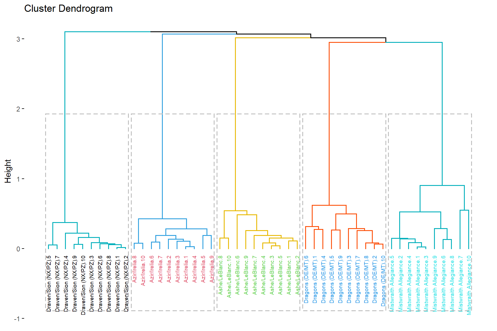
With the hierarchical clustering we have can not only how clearly the method grouped the archetypes but the similarities between the groups and how some archetypes may suggest the presence of sub-archetypes similarly by how we choose them, at least for Dragons and Sion. As Mistwraith decks contain an higher range in similarity cutting the dendogram in more than 5 archetypes would first and foremost identify the differences in SI decks.
Overall the methods can provide a useful tool to explore the cluster but suffer from the fact that it doesn’t scale well at the increase of sample size, not just in term of memory/cost but as how to find a proper level to cut the tree.
K-Medoid
The K-Medoid applied with 5 cluster had the same results of all the other methods but differently from the other it was able to identify a couple of the Marauder decks when he used 7 clusters. As the more interesting result, we will report the one with 7 cluster.
| 1 | 2 | 3 | 4 | 5 | 6 | 7 | |
|---|---|---|---|---|---|---|---|
| Ashe/LeBlanc | 7 | 0 | 0 | 0 | 0 | 0 | 0 |
| Azir/Irelia | 0 | 0 | 10 | 0 | 0 | 0 | 0 |
| Dragons | 0 | 0 | 0 | 7 | 0 | 0 | 0 |
| Dragons+J4 | 0 | 0 | 0 | 3 | 0 | 0 | 0 |
| Draven/Sion | 0 | 0 | 0 | 0 | 8 | 0 | 0 |
| Marauder | 1 | 2 | 0 | 0 | 0 | 0 | 0 |
| Mistwraith(MT) | 0 | 0 | 0 | 0 | 0 | 5 | 0 |
| Mistwraith(PnZ) | 0 | 0 | 0 | 0 | 0 | 4 | 1 |
| RubinBait-Sion | 0 | 0 | 0 | 0 | 2 | 0 | 0 |
With K-Medoids the algorithm also provide the examplars that identified correctly most (2/3) of the Marauder decks and assigned the Mistwraith-Viego deck to its own cluster.
| archetype | archetype.v2 | deck_code |
|---|---|---|
| Ashe/LeBlanc | Ashe/LB | |
| Ashe/LeBlanc/Sejuani | Marauder | |
| Azir/Irelia | Azir/Irelia | |
| Aurelion Sol/Shyvana | Dragons | |
| Draven/Sion (NX/PZ) | Dragon/Sion | |
| Elise/Kalista (MT/SI) | Mistwraith | |
| Viego (PZ/SI) | Mistwraith |
DBSCAN
As DBSCAN also introduce noise points we want to check which points have been assigned as such.
Not surprisingly the noise was found in the Mistwraith decks always including as noise the ‘Viego’ variant. With DBSCAN we have to remember it could be wiser to test for a wider range of hyper-parameters minPts and \(\epsilon\).
Yet, the main cons of this method is exactly how to define minPts, especially if we used a bigger/real dataset as we have no idea about the distribution of the archetypes lists.
Overall this method can be a valuable source to check for outliers in the archetypes list but we are not sure its definition of noise of appropriate for the archetype problem.
| 0 | 1 | 2 | 3 | 4 | 5 | |
|---|---|---|---|---|---|---|
| Ashe/LeBlanc | 0 | 9 | 0 | 0 | 0 | 0 |
| Ashe/LeBlanc/Sejuani | 0 | 1 | 0 | 0 | 0 | 0 |
| Aurelion Sol/Jarvan IV/Shyvana | 0 | 0 | 0 | 3 | 0 | 0 |
| Aurelion Sol/Shyvana | 0 | 0 | 0 | 7 | 0 | 0 |
| Azir/Irelia | 0 | 0 | 10 | 0 | 0 | 0 |
| Draven/Sion (NX/PZ) | 0 | 0 | 0 | 0 | 10 | 0 |
| Elise/Kalista (MT/SI) | 0 | 0 | 0 | 0 | 0 | 4 |
| Elise/Kalista (PZ/SI) | 0 | 0 | 0 | 0 | 0 | 2 |
| Kalista (PZ/SI) | 1 | 0 | 0 | 0 | 0 | 1 |
| Kalista/Nocturne (MT/SI) | 0 | 0 | 0 | 0 | 0 | 1 |
| Viego (PZ/SI) | 1 | 0 | 0 | 0 | 0 | 0 |
| 0 | 1 | 2 | 3 | 4 | 5 | |
|---|---|---|---|---|---|---|
| Ashe/LeBlanc | 0 | 9 | 0 | 0 | 0 | 0 |
| Ashe/LeBlanc/Sejuani | 0 | 1 | 0 | 0 | 0 | 0 |
| Aurelion Sol/Jarvan IV/Shyvana | 0 | 0 | 0 | 3 | 0 | 0 |
| Aurelion Sol/Shyvana | 0 | 0 | 0 | 7 | 0 | 0 |
| Azir/Irelia | 0 | 0 | 10 | 0 | 0 | 0 |
| Draven/Sion (NX/PZ) | 0 | 0 | 0 | 0 | 10 | 0 |
| Elise/Kalista (MT/SI) | 0 | 0 | 0 | 0 | 0 | 4 |
| Elise/Kalista (PZ/SI) | 0 | 0 | 0 | 0 | 0 | 2 |
| Kalista (PZ/SI) | 0 | 0 | 0 | 0 | 0 | 2 |
| Kalista/Nocturne (MT/SI) | 0 | 0 | 0 | 0 | 0 | 1 |
| Viego (PZ/SI) | 1 | 0 | 0 | 0 | 0 | 0 |
Lastly, when considering DBSCAN there is a monumental reason why the method may be not yet appropriate to use.
As described DBSCAN is based on the idea if clusters separated by region with different density of data points. As of now we are not sure if the archetype problem can truly satisfy this requirement as the card pool in Legends of Runeterra is extremely limited compared to counterparts like Magic: the Gathering or Yu-Gi-Oh.
APcluster
Lastly the APcluster algorithm
| 7 | 17 | 28 | 36 | 48 | |
|---|---|---|---|---|---|
| Ashe/LeBlanc | 7 | 0 | 0 | 0 | 0 |
| Azir/Irelia | 0 | 10 | 0 | 0 | 0 |
| Dragons | 0 | 0 | 7 | 0 | 0 |
| Dragons+J4 | 0 | 0 | 3 | 0 | 0 |
| Draven/Sion | 0 | 0 | 0 | 8 | 0 |
| Marauder | 3 | 0 | 0 | 0 | 0 |
| Mistwraith(MT) | 0 | 0 | 0 | 0 | 5 |
| Mistwraith(PnZ) | 0 | 0 | 0 | 0 | 5 |
| RubinBait-Sion | 0 | 0 | 0 | 2 | 0 |
The column names refers to the id of the examplars chosen to represent the archetype
(#fig:heat-apcluster.v2)Heatmap with labels obtained by applying APcluster to the example data set
As now it could be expected the ‘less homogeneous’ cluster was the one from Mistwraith decks.
If we wanted we can apply an agglomerative clustering on top of AP clustering.
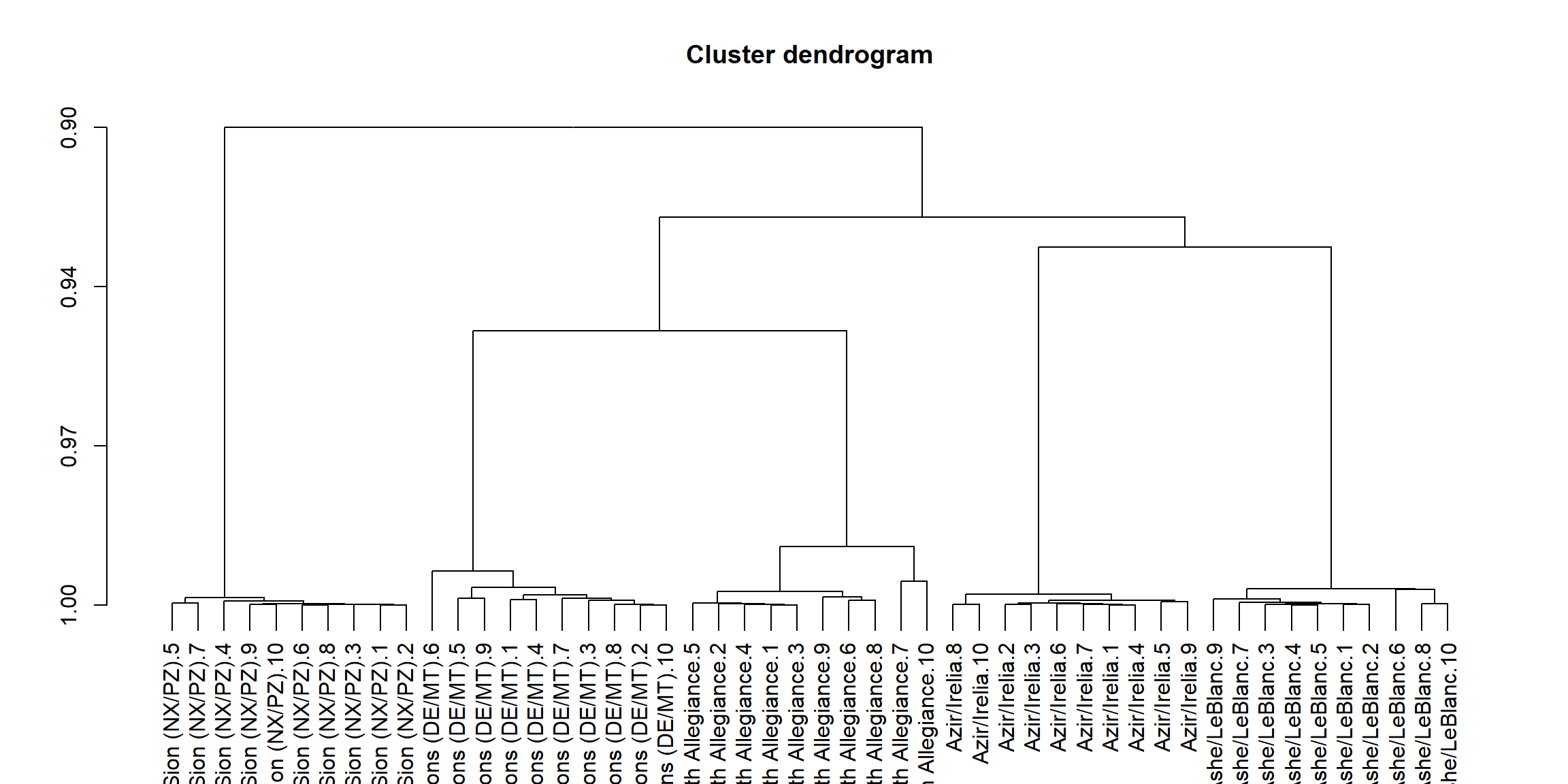
Figure 11: Dendogram obtained by applying APcluster to the example data set
And lastly as K-Medoid we can see the examplars provided by the algorithm
| archetype | archetype.v2 | deck_code |
|---|---|---|
| Ashe/LeBlanc | Ashe/LB | |
| Azir/Irelia | Azir/Irelia | |
| Aurelion Sol/Shyvana | Dragons | |
| Draven/Sion (NX/PZ) | Dragon/Sion | |
| Elise/Kalista (PZ/SI) | Mistwraith |
Again, the Burn variant of Draven/Sion looks way confounded in its own archetype, the remaining results are similar to the other methods. The results could overall be more optimized of affinity propagation clustering is an extremely flexible method but we lack for now experience with it.
Conclusion
Clustering is truly a wide and troublesome (and fascinating) domain. As there is no clear definition about how to define an archetype in Legends of Runeterra finding an appropriate approach to classify them based on clustering analysis is no easy task.
While most cluster algorithm used in this articles were able to differentiate for the macro-archetypes selected for this example the example of Draven/Sion decks shows that some variant that is recognized by the community as a different deck.
A better definition of the problem seems to be crucial in order to approach the archetype problem as, as of now it mostly relies on intuition and shared agreements about how to consider certain decks.
Even if the results did agreed for the most part among all the algorithm the degree of freedom left to the user that could hinder the results has to be taken into account for which methods are worth exploring with bigger/real examples. K-Means is the method that overall we would consider the worst as it’s affect by the randomized initialisation step, the choice of k-cluster that is guided ‘not as good’ as the methods that can provide dendograms or exemplars to further explore the choices and results. K-Medoids while a more robust version of K-Means still suffer from the initialisation step. Hierarchical clustering another basic clustering algorithm is a promising option to check for possible sub-archetypes or differences within cluster. The main concern is the scale with bigger data-set as the required dissimilarity matrix has a quadratic increase of the sample size.
Legal bla bla
This content was created under Riot Games’ “Legal Jibber Jabber” policy using assets owned by Riot Games. Riot Games does not endorse or sponsor this project.
as we use a sparse matrix that contain the number of copies for each card, so with possible value \([0,3] \in \mathbb{N}\), in this example, no it’s not necessary to standardize↩︎
Not exactly: for k = n the wss is not even defined as it’s not possible to define variance for n=1.↩︎
This behaviour allows AHC to more easily identify smaller clusters. In contrast, Divisive Hierarchical clustering is more robust to noise and outliers.↩︎
I’m sorry to say I wasn’t clear in the first draft that \(\epsilon\) wasn’t the same after using a different metric. Let me also add that trying to use the elbow method with the manhattan distance proved to be quite ineffective and the ‘logical’ choice of 3 cards differences worked much better.↩︎